J. Li and M. Guo
School of Computer Science and Technology, Harbin Institute of Technology, Harbin, China
Corresponding author: J. Li
E-mail: [email protected] or [email protected]

Genet. Mol. Res. 6 (3): 522-533 (2007)
Received March 9, 2007
Accepted June 22, 2007
Published September 5, 2007

ABSTRACT. The evolutionary tree reconstruction algorithm called SEMPHY using structural expectation maximization (SEM) is an efficient approach but has local optimality problem. To improve SEMPHY, a new algorithm named HSEMPHY based on the homotopy continuation principle is proposed in the present study for reconstructing evolutionary trees. The HSEMPHY algorithm computes the condition probability of hidden variables in the structural through maximum entropy principle. It can reduce the influence of the initial value of the final resolution by simulating the process of the homotopy principle and by introducing the homotopy parameter β. HSEMPHY is tested on real datasets and simulated dataset to compare with SEMPHY and the two most popular reconstruction approaches PHYML and RAXML. Experimental results show that HSEMPHY is at least as good as PHYML and RAXML and is very robust to poor starting trees.

Key words: Evolutionary tree reconstruction, Maximum likelihood, Structural expectation maximization, Homotopy method

INTRODUCTION

The inference of phylogenies with computational methods has many important applications in medical and biological research, such as drug discovery and conservation biology. Well-known techniques for phylogeny analysis include distance-based methods such as neighbor-joining, maximum parsimony, and maximum likelihood (ML). A number of studies (Rosenberg and Kumar, 2001; Ranwez and Gascuel, 2002) have shown that ML programs can recover the correct tree from simulated data sets more frequently than other methods can, which supported numerous observations from real data and explains their popularity.

However, the disadvantage of ML methods is that they require considerable computational effort. The fundamental algorithmic problems involve an immense amount of potential tree topologies. This number grows exponentially with the number of sequences n, e.g., for n = 50 organisms there exist already 2.84 x 10⁷⁶ alternative topologies; a number almost as large as the number of atoms in the universe (≈10⁸⁰). On the other hand, even computing the optimal values of edge lengths on a single tree is not an easy task. This requires cumbersome numerical optimization techniques simply due to the number of parameters (2n-3 edges, where n is the number of sequences). In fact, it has already been demonstrated that finding the optimal tree under the ML criterion is NP-hard (Roch, 2006). Consequently, the introduction of heuristics becomes inevitable.

Research in ML presently focuses on two points. One is on search strategies to reduce the search space in terms of potential tree topologies evaluated. For example, hill climbing-based reconstruction algorithms (Felsenstein, 1993; Olsen et al., 1994; Wolf et al., 2000; Guindon and Gascuel, 2003); simulated annealing-based reconstructions (Salter and Pearl, 2001); genetic algorithm-based reconstructions (Lewis, 1998; Lemmon and Milinkovitch, 2002; Brauer et al., 2002; Zwickl, 2006); Markov chain Monte Carlo algorithms are widely used in Bayesian methods (Rannala and Yang, 1996; Li et al., 2000; Simon and Larget, 2000; Huelsenbeck and Ronquist, 2001). The other is on the technical issues of the calculation of ML (Kosakovsky Pond and Muse, 2004; Stamatakis, 2002, 2006).

However, despite that many efforts have been made in the last decades, inference of evolutionary trees using the ML method is far from satisfactory (Williams and Moret, 2003), which greatly frustrates many researchers.

On the other hand, Friedman et al. presented in 2002 an evolutionary tree reconstruction using structural expectation maximization (SEM; Friedman, 1998) for the first time and achieved some success, which provided a new direction in the research of phylogeny reconstruction. SEM is very efficient in estimating model structures using ML with incomplete data. Starting from a structure, SEM completes the data iteratively and probabilistically, according to the distribution induced by the current model, and uses the completed data to evaluate different candidate structures. The merit of SEM includes reliable global convergence, low cost per iteration and easy programming.

However, in SEM, the condition probability of the hidden variables is directly computed by Bayes’ rule and the structure obtained in every iteration is optimized with respect to the expected likelihood value of the optima in the last iteration. As a result, in later iterations of the procedure, the trees that maximize this expected likelihood value will tend to be similar to the tree found in the previous iteration. Furthermore, this self-bias gives rise to stationary points of SEM iterations. Moreover, theoretical (Steel, 1994) as well as empirical evidence using simulated (Rogers and Swofford, 1999; Chor et al., 2000) and real (Salter and Pearl, 2001) data has demonstrated that multiple maxima exist under ML. Therefore, the reconstruction algorithm using SEM such as SEMPHY can often be strapped in local optima.

The homotopy method belongs to the field of global optimization techniques (Wu, 1996). The main idea is that a smoothed version of the objective function is first optimized. With enough smoothing, the optimization will be convex and the global optimum can be found. Smoothing then increases and the new optima are computed, where the solution found in the previous step serves as a starting point. The algorithm iterates until there is no smoothing. The illustration of the homotopy continuation method is shown in Figure 1.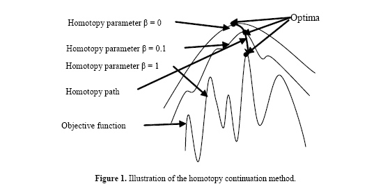

To escape from local optima, this paper further enhances the SEMPHY by simulating the process of the homotopy principle. The new reconstruction algorithm called HEMPHY optimizes a series of smoothed versions of the objective functions with different homotopy parameter β but not the objective function directly. With enough small β, the global optima can be found without the influence of the initial value. β then increases and the new optima are computed, where the solution found in the previous step serves as a starting point. Thus, with the increase of β, HEMPHY can finally converge on the global optimum of the objective likelihood function.

The remainder of the article is organized as follows. Section 2 reviews the ML and SEM algorithms. Section 3 gives the derivation of the new SEM algorithm called HSEM. Section 4 details the evolutionary tree reconstruction algorithm HSEMPHY using HSEM. Section 5 compares HSEMPHY with SEMPHY and the two popular reconstruction approaches through experiments and concludes this paper.

Maximum likelihood and SEM algorithm

In terms of graph theory, a rooted evolutionary tree is a binary tree. Branch lengths of each edge in the graph represent evolutionary distances, which is a measure of how close (or different) sequences are. Internal nodes in the tree represent hypothetical ancestors, which evolved into distinct descendants. The leaves of the tree represent known sequences.

Given a dataset D_n×m containing n sequences with m sites, the main idea of ML is to find a tree T with highest likelihood value P(D|T,t) or log P(D|T,t), where T and t represent the branch pattern and the branch length of the evolutionary tree T, respectively.

The likelihood function of an evolutionary tree is based on a model of evolution. To simplify computations, the current models are generally assumed to have the two properties as follows:

• All sites evolve identically and independently. Thus, the likelihood for all sites is the product of the likelihoods for individual sites.

• Evolution is time reversible, that is

where p_i denotes the probability of state i,

denotes the time undergone from state i to state j , and

denotes the probability of state i becoming state j after t_ij .

The likelihood function of the whole dataset D given the phylogeny (T,t) is then defined as follows:

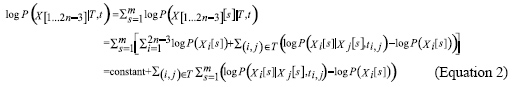
According to ML, we need to find a topology T and associated parameters t that maximizes this likelihood. The evolutionary tree (T,t) is, in some sense, the most plausible candidate for having generated the data.

Even for simple models of evolution (parsimony), and for a binary alphabet, the problem has been shown to be NP-hard since there are n-3 internal nodes that are unknown, and we need to jointly optimize over the parameters. For general stochastic models, no polynomial granted optimization algorithm is known even for a fixed topology (Rambaut and Grassly, 1997). Even heuristics are often too computationally intensive for all but small data sets. All this has led to the situation that, although it has been shown that ML produces more accurate results, researchers are forced to use some other optimization criterion instead of ML for real life applications.

However, when internal nodes are assumed known, the likelihood of the complete data is

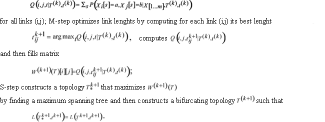
As shown in Equation 2, in case of complete data, the global optimization problem breaks down into significantly smaller problems, where we optimize the parameters of each independent of the rest. The ML problem is reduced to a combinatorial optimization problem, which greatly decreases the computation complexity.

Therefore, to decrease the computation complexity, P(D|T,t) can be approached through P(D,H|T,t). This is the proper idea of SEM.

SEM is very efficient for estimating model structures using ML with incomplete data. Starting from a structure, SEM iteratively and probabilistically completes the data according to the distribution induced by the current model and uses the completed data to evaluate different candidate structures. Each iteration of the SEM algorithm consists of three processes: the E-step, the M-step and the S-step. In the E-step, the hidden data are estimated given the observed data and current estimate of the model and parameters. This is achieved using the conditional expectation, explaining the choice of terminology. In the M-step, the likelihood function is maximized under the assumption that the missing data are known. The estimates of the missing data from the E-step are used in lieu of the actual hidden data. In the S-step, the structure is adjusted according to the parameters estimated in M-step. Convergence is assured since the algorithm guarantees the increase in the likelihood value at each iteration. The main idea of the SEM-based evolutionary tree reconstruction algorithm called SEMPHY, introduced by Friedman, is that in the (k + 1)th iteration, E-step computes expectation

However, in SEM, the condition probability of the hidden variables is directly computed by Bayes’ rule and the structure obtained in every iteration is optimized with respect to the expected likelihood value of the optima in the last iteration. As a result, in later iterations of the procedure, the trees that maximize this expected likelihood value will tend to be similar to the tree found in the previous iteration. Furthermore, this self-bias gives rise to stationary points of SEM iterations. This makes the performance of SEM depend on its starting point. To improve SEMPHY, a new algorithm named HSEMPHY based on the homotopy principle is proposed in this paper for reconstructing evolutionary trees. The HSEMPHY algorithm computes the condition probability of the hidden variable in the structural through maximum entropy principle. It can reduce the influence of the initial value on the final resolution by simulating the process of the homotopy continuation principle to resolve problems and by introducing the homotopy parameter β. The problem to get trapped in local optima is also then overcome.

HSEM algorithm

Let y be observed variables, z be unobserved variables and θ be parameters to be estimated in model structure M^k. In case of compute data x = (y,z), the likelihood function log p (z,y|θ, M^k) can be seen as the function of the hidden variables z for fixed model structure M^k and parameter θ.

In the kth iteration, the conditional probability of z in M^k is assumed as f(z|y,Θ,M^k). According to the maximum entropy principle, we need to maximize the entropy

with respect to f(z|y,Θ,M^k) subject to the constraints of Equations 3 and 4.

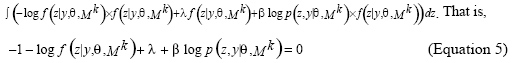
According to the variation principle, the objective function is

From Equation 5, we can obtain Equation 6 as follows.

Replace in Equation 3 with Equation 6, we can arrive at

From Equations 6 and 7, thus

where β is the homotopy parameter.

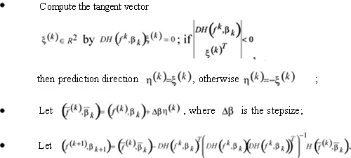
We can adopt the prediction-correction method to trace the homotopy path as the parameter β varies from 0 to 1.The procedure is shown as follows:

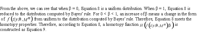
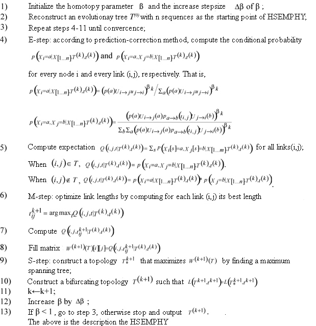
The above is the derivation of HSEM. We can see that HSEM adds a homotopy-loop to the original SEM algorithm and replaces the condition probability of hidden variables originally computed by Bayes' rule with Equation 8. When β is very small, the dependency of HSEM iterations on the starting point is very weak; as the iterations proceed, β increases, the dependency of HSEM iterations on the starting point becomes increasingly stronger. When β = 1, HSEM tries to determine ML precisely. When the parameter β is initialized as 1, HSEM is reduced to SEM, that is, SEM is a special case of HSEM. Therefore, in theory, the optimum returned by HSEM is at least as good as that by SEM.

Evolutionary tree reconstruction using HSEM

On the basis of SEMPHY, introduced by Friedman, this paper presents an evolutionary tree reconstruction algorithm called HSEMPHY using HSEM. A significant difference between HSEMPHY and SEMPHY is that HSEMPHY is multiple iterations of the SEMPHY procedure with different parameter β. When β is increased to some size (β ≥ 1) and convergence conditions are met, HSEMPHY stops.

The pseudocode of the HSEMPHY is shown as follows.

Input: a dataset D of n sequences with m sites

Output: a phylogeny of D

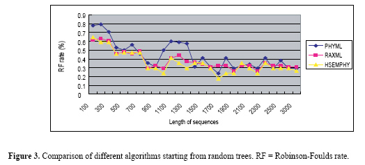
Experiments

In this section, HSEMPHY is tested through experiments. The experiments include two parts. In the first part, HSEMPHY is compared with SEMPHY to test the robustness to starting points. In the second part, HSEMPHY is compared with the two most popular algorithms, PHYML, and RAXML to test the efficiency of HSEMPHY. Two versions of all algorithms are tested. One version is started from relatively better evolutionary trees (reconstructed by reconstruction algorithms such as neighbor joining), the other version is started from random trees. Random trees are useful to check that the algorithm is not affected by potentially poor starting trees, while starting with relatively better evolutionary trees corresponds to standard use, notably regarding efficiency.

All the algorithms are also based on the HKY85 nucleotide substitution model with a transition/transversion ratio of 2.0, plus a four-category discrete gamma distribution of parameter 0.3. The frequencies of every nucleotide are empirical frequencies estimated from sequences. In addition, the stepsize increase of homotopy parameter β is 0.2.

Comparison of HSEMPHY with SEMPHY

To test the sensitivity to the starting points, HSEMPHY is tested on 10 real datasets, such as lysozymeSmall, TipDate, lysozymeLarge, CatLemurs, Rbcl55, 101_SC, 4Dat, 3dat, 132, and 150_ARB, to compare its result and that of SEMPHY. Experimental results are shown in Table 1.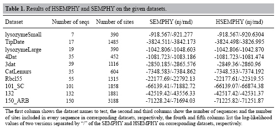

From Table 1, we can see that when starting from neighbor joining trees, HSEMPHY is at least as good as SEMPHY; while starting from random trees, HSEMPHY is better than SEMPHY, which means that HSEMPHY is robust to poor starting points.

Comparison of HSEMPHY with two most popular algorithms

HSEMPHY is tested on both simulated and real datasets mentioned in the "Comparison of HSEMPHY with SEMPHY" subtitle to compare with the two most popular methods, PHYML and RAXML.

Tests on simulated datasets

In computer simulation experiments, an important measure criterion is the Robinson-Foulds (RF) rate which measures the topological difference between two evolutionary trees.

Twenty-eight datasets of 40 sequences with different lengths generated by Seq-gen[29] are tested in this experiment. The results are shown in Figures 2 and 3.

From Figure 2, we can see that when three algorithms are all started from relatively better trees, none of the algorithms is always better than any of the other two algorithms in all datasets. On some datasets, HSEMPHY is better than others; however, on some datasets, PHYML (RAXML) is better than others.

From Figure 3, we can see that the difference in the performance of three algorithms is distinct, where PHYML is the worst, RAXML is better and the HSEMPHY is the best.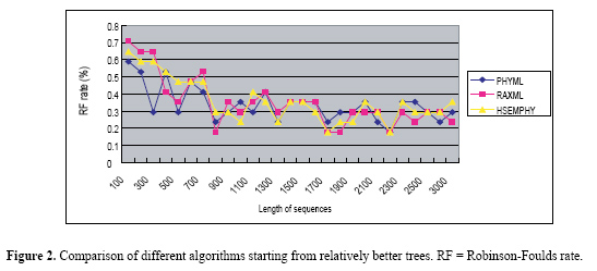

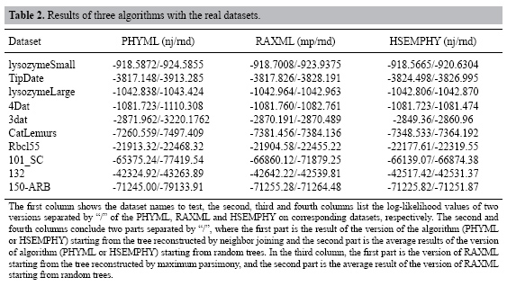
Tests on real datasets

HSEMPHY, PHYML and RAXML are compared on 10 real datasets mentioned in the "Comparison of HSEMPHY with SEMPHY" subtitle. To improve the speed, both PHYML and RAXML have adopted some specific technical strategy. Therefore, a direct comparison of running times of these three algorithms, although useful for practical purposes, does not give much insight into the improvements in efficiency that is achieved by our proposed method. Consequently, we only care about the quality of the resulting evolutionary tree. Moreover, since there is a difference in the way likelihood values are calculated among PHYML, RAXML and HSEMPHY, final trees found by PHYML and RAXML are reevaluated using PHYML (without doing any further optimization, but just evaluating the likelihood of the given tree) to enable a direct comparison.

The experimental results are shown in Table 2.

From Table 2, we can see that when starting from a relatively better tree, HSEMPHY is comparable with PHYML and RAXML; while starting from random trees, HSEMPHY is the better than PHYML and RAXML.

From the above experiments, it can be concluded that that HSEMPHY is at least as good as the PHYML and RAXML and is very robust to poor starting trees.

ACKNOWLEDGMENTS

Research supported by the Natural Science Foundation of China under Grant No. 60671011, the Science Fund for Distinguished Young Scholars of Heilongjiang Province in China under Grant No. JC200611, the Science and Technology Fund for Returnee of Heilongjiang Province in China, and Foundation of Harbin Institute of Technology under Grant No. HIT.2003.53.

REFERENCES

Brauer MJ, Holder MT, Dries LA, Zwickl DJ, et al. (2002). Genetic algorithms and parallel processing in maximum-likelihood phylogeny inference. Mol. Biol. Evol. 19: 1717-1726.

Chor B, Hendy MD, Rolland BR and Penny D (2000). Multiple maxima of likelihood in phylogenetic trees: an analytic approach. Mol. Biol. Evol. 17: 1529-1541.

Felsenstein J (1993). PHYLIP (phylogeny inference package), version 3.6a2. Distributed by the author, Department of Genetics, University of Washington, Seattle.

Friedman N (1998). The Bayesian structural EM algorithm. In: Proceedings of the 14th Conference on Uncertainty in AI. Morgan Kaufmann, San Francisco, 129-138.

Friedman N, Ninio M, Pe’er I and Pupko T (2002). A structural EM algorithm for phylogenetic inference. J. Comput. Biol. 9: 331-353.

Guindon S and Gascuel O (2003). A simple, fast, and accurate algorithm to estimate large phylogenies by maximum likelihood. Syst. Biol. 52: 696-704.

Huelsenbeck JP and Ronquist F (2001). MrBayes: Bayesian inference of phylogenetic trees. Bioinformatics 17: 754-755.

Kosakovsky Pond SL and Muse SV (2004). Column sorting: rapid calculation of the phylogenetic likelihood function. Syst. Biol. 53: 685-692.

Lemmon AR and Milinkovitch MC (2002). The metapopulation genetic algorithm: an efficient solution for the problem of large phylogeny estimation. Proc. Natl. Acad. Sci. USA 99: 10516-10521.

Lewis PO (1998). A genetic algorithm for maximum-likelihood phylogeny inference using nucleotide sequence data. Mol. Biol. Evol. 15: 277-283.

Li S, Pearl D and Doss H (2000). Phylogenetic tree construction using Markov chain Monte Carlo. J. Am. Stat. Assoc. 95: 493-508.

Olsen GJ, Matsuda H, Hagstrom R and Overbeek R (1994). fastDNAmL: a tool for construction of phylogenetic trees of DNA sequences using maximum likelihood. Comput. Appl. Biosci. 10: 41-48.

Rambaut A and Grassly NC (1997). Seq-Gen: an application for the Monte Carlo simulation of DNA sequence evolution along phylogenetic trees. Comput. Appl. Biosci. 13: 235-238.

Rannala B and Yang Z (1996). Probability distribution of molecular evolutionary trees: a new method of phylogenetic inference. J. Mol. Evol. 43: 304-311.

Ranwez V and Gascuel O (2002). Improvement of distance-based phylogenetic methods by a local maximum likelihood approach using triplets. Mol. Biol. Evol. 19: 1952-1963.

Rice K and Warnow T (1997). Parsimony is hard to beat. Proceedings of the 3rd Annual International Conference on Computing and Combinatorics, Shanghai, 124-133.

Roch S (2006). A short proof that phylogenetic tree reconstruction by maximum likelihood is hard. IEEE/ACM Trans. Comput. Biol. Bioinform. 3: 92-94.

Rogers JS and Swofford DL (1999). Multiple local maxima for likelihoods of phylogenetic trees: a simulation study. Mol. Biol. Evol. 16: 1079-1085.

Rosenberg MS and Kumar S (2001). Traditional phylogenetic reconstruction methods reconstruct shallow and deep evolutionary relationships equally well. Mol. Biol. Evol. 18: 1823-1827.

Salter LA and Pearl DK (2001). Stochastic search strategy for estimation of maximum likelihood phylogenetic trees. Syst. Biol. 50: 7-17.

Simon D and Larget B (2000). Bayesian analysis in molecular biology and evolution (BAMBE), version 2.03beta. Department of Mathematics and Computer Science, Duquesne University, Pittsburgh.

Stamatakis A (2006). RAxML-VI-HPC: maximum likelihood-based phylogenetic analyses with thousands of taxa and mixed models. Bioinformatics 22: 2688-2690.

Stamatakis A, Ludwig T, Meier H and Wolf MJ (2002). AxML: a fast program for sequential and parallel phylogenetic tree calculations based on the maximum likelihood method. In: Proceedings of 1st IEEE Computer Society Bioinformatics Conference (CSB2002), Stanford University, Palo Alto, 21-28.

Steel M (1994). The maximum likelihood point for a phylogenetic tree is not unique. Syst. Biol. 43: 560-564.

Williams TL and Moret BME (2003). An investigation of phylogenetic likelihood methods. Proceedings of the 3rd IEEE Symposium on BioInformatics and BioEngineering (BIBE’03), Albuquerque, 79-86.

Wolf MJ, Easteal S, Kahn M, McKay BD, et al. (2000). TrExML: a maximum-likelihood approach for extensive tree-space exploration. Bioinformatics 16: 383-394.

Wu Z (1996). The effective energy transformation scheme as a special continuation approach to global optimization with application to molecular conformation. SIAM J. Optimization 6: 748-768.

Zwickl DJ (2006). Genetic algorithm approaches for the phylogenetic analysis of large biological sequence datasets under the maximum likelihood criterion. Ph.D. dissertation, The University of Texas, Austin.